MachineLearning스터디/LinearRegressionWithMultipleVariables: Difference between revisions
From ZeroWiki
More actions
imported>trailblaze No edit summary |
imported>trailblaze No edit summary |
||
| (6 intermediate revisions by the same user not shown) | |||
| Line 1: | Line 1: | ||
__TOC__ | __TOC__ | ||
* 모든 것을 정리하려고 하니 효율이 떨어진다. 중요하다 생각되는 것만 우선 정리하기로.. | |||
* 이 문서에 있는 사진이나 예제의 상당수는 [https://www.coursera.org/course/ml Coursera/ML강의]에 남겨져 있음. PPT도 제공하므로 꼭 확인하세요. | |||
=== Multiple Features === | === Multiple Features === | ||
=== Gradient Descent for Multiple Variables === | === Gradient Descent for Multiple Variables === | ||
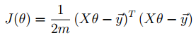
==== Cost Function ==== | |||
[[File:CostFunctionWithMultipleVariables.PNG]] | |||
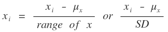
=== Feature Scaling === | === Feature Scaling === | ||
[[File:Mean_Normalization.png]] | |||
=== Learning Rate === | === Learning Rate === | ||
=== Polynomial Regression === | === Polynomial Regression === | ||
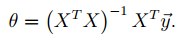
=== Normal Equation === | === Normal Equation === | ||
[[File:Normal_Equation.PNG]] | |||
=== 정리 === | |||
==== Gradient Descent ==== | |||
* Learning Rate α를 잘 정하는게 중요. | |||
* Feature의 수가 클 때 사용. (100000개 이상) | |||
==== Normal Equation ==== | |||
* [[File:invert.png]] 의 계산이 필요. O(N^3)의 시간복잡도를 가짐. | |||
* Feature의 수가 적을 때 사용. (10000개 까지) | |||
=== Octave로 Linear Regression With Multiple Varables 구현하기 === | === Octave로 Linear Regression With Multiple Varables 구현하기 === | ||
==== Feature Normalize ==== | |||
function [X_norm, mu, sigma] = featureNormalize(X) | |||
%FEATURENORMALIZE Normalizes the features in X | |||
% FEATURENORMALIZE(X) returns a normalized version of X where | |||
% the mean value of each feature is 0 and the standard deviation | |||
% is 1. This is often a good preprocessing step to do when | |||
% working with learning algorithms. | |||
% You need to set these values correctly | |||
X_norm = X; | |||
mu = zeros(1, size(X, 2)); | |||
sigma = zeros(1, size(X, 2)); | |||
n_of_feature = size(X_norm, 2); | |||
for i = 1:n_of_feature | |||
mu(i) = mean(X_norm(:, i)); | |||
sigma(i) = std(X_norm(:, i)); | |||
X_norm(:, i) = (X_norm(:, i ) - mu(i)) / sigma(i); | |||
end | |||
* mean : 평균 구하는 함수. | |||
* std : 표준 편차 구하는 함수. | |||
* 표준 편차를 이용해서 데이터를 정규화 시킴. | |||
==== Compute Cost ==== | |||
function J = computeCostMulti(X, y, theta) | |||
%COMPUTECOSTMULTI Compute cost for linear regression with multiple variables | |||
% J = COMPUTECOSTMULTI(X, y, theta) computes the cost of using theta as the | |||
% parameter for linear regression to fit the data points in X and y | |||
% Initialize some useful values | |||
m = length(y); % number of training examples | |||
% You need to return the following variables correctly | |||
J = 0; | |||
% ====================== YOUR CODE HERE ====================== | |||
% Instructions: Compute the cost of a particular choice of theta | |||
% You should set J to the cost. | |||
J = (X * theta - y)' * (X * theta - y) / (2 * m); | |||
% ========================================================================= | |||
end | |||
* 왜 이게 되는지는 모르겠음. 아는 사람은 추가바람. | |||
==== Gradient Descent ==== | |||
function [theta, J_history] = gradientDescentMulti(X, y, theta, alpha, num_iters) | |||
%GRADIENTDESCENTMULTI Performs gradient descent to learn theta | |||
% theta = GRADIENTDESCENTMULTI(x, y, theta, alpha, num_iters) updates theta by | |||
% taking num_iters gradient steps with learning rate alpha | |||
% Initialize some useful values | |||
m = length(y); % number of training examples | |||
J_history = zeros(num_iters, 1); | |||
for iter = 1:num_iters | |||
temp = theta; | |||
E = X * theta - y; | |||
for j=1:size(X, 2) | |||
delta = sum(E .* X(:, j)) / m; | |||
temp(j, 1) = temp(j, 1) - alpha * delta; | |||
end | |||
theta = temp; | |||
% ====================== YOUR CODE HERE ====================== | |||
% Instructions: Perform a single gradient step on the parameter vector | |||
% theta. | |||
% | |||
% Hint: While debugging, it can be useful to print out the values | |||
% of the cost function (computeCostMulti) and gradient here. | |||
% | |||
% ============================================================ | |||
% Save the cost J in every iteration | |||
J_history(iter) = computeCostMulti(X, y, theta); | |||
end | |||
---- | |||
[[MachineLearning스터디]] | |||
Latest revision as of 03:40, 18 February 2014
- 모든 것을 정리하려고 하니 효율이 떨어진다. 중요하다 생각되는 것만 우선 정리하기로..
- 이 문서에 있는 사진이나 예제의 상당수는 Coursera/ML강의에 남겨져 있음. PPT도 제공하므로 꼭 확인하세요.
Multiple Features
Gradient Descent for Multiple Variables
Cost Function

Feature Scaling

Learning Rate
Polynomial Regression
Normal Equation
정리
Gradient Descent
- Learning Rate α를 잘 정하는게 중요.
- Feature의 수가 클 때 사용. (100000개 이상)
Normal Equation
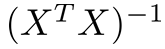 의 계산이 필요. O(N^3)의 시간복잡도를 가짐.
- Feature의 수가 적을 때 사용. (10000개 까지)
Octave로 Linear Regression With Multiple Varables 구현하기
Feature Normalize
function [X_norm, mu, sigma] = featureNormalize(X)
%FEATURENORMALIZE Normalizes the features in X
%   FEATURENORMALIZE(X) returns a normalized version of X where
%   the mean value of each feature is 0 and the standard deviation
%   is 1. This is often a good preprocessing step to do when
%   working with learning algorithms.

% You need to set these values correctly
X_norm = X;
mu = zeros(1, size(X, 2));
sigma = zeros(1, size(X, 2));
n_of_feature = size(X_norm, 2);
for i = 1:n_of_feature
	mu(i) = mean(X_norm(:, i));
	sigma(i) = std(X_norm(:, i));
	X_norm(:, i) = (X_norm(:, i ) - mu(i)) / sigma(i);
end
- mean : 평균 구하는 함수.
- std : 표준 편차 구하는 함수.
- 표준 편차를 이용해서 데이터를 정규화 시킴.
Compute Cost
function J = computeCostMulti(X, y, theta)
%COMPUTECOSTMULTI Compute cost for linear regression with multiple variables
%   J = COMPUTECOSTMULTI(X, y, theta) computes the cost of using theta as the
%   parameter for linear regression to fit the data points in X and y

% Initialize some useful values
m = length(y); % number of training examples

% You need to return the following variables correctly
J = 0;

% ====================== YOUR CODE HERE ======================
% Instructions: Compute the cost of a particular choice of theta
%               You should set J to the cost.
J = (X * theta - y)' * (X * theta - y) / (2 * m);


% =========================================================================

end
- 왜 이게 되는지는 모르겠음. 아는 사람은 추가바람.
Gradient Descent
function [theta, J_history] = gradientDescentMulti(X, y, theta, alpha, num_iters)
%GRADIENTDESCENTMULTI Performs gradient descent to learn theta
%   theta = GRADIENTDESCENTMULTI(x, y, theta, alpha, num_iters) updates theta by
%   taking num_iters gradient steps with learning rate alpha
% Initialize some useful values
m = length(y); % number of training examples
J_history = zeros(num_iters, 1);
for iter = 1:num_iters
	temp = theta;
	E = X * theta - y;
	for j=1:size(X, 2)
		delta = sum(E .* X(:, j)) / m;
		temp(j, 1) = temp(j, 1) - alpha * delta;
	end
	theta = temp;
    % ====================== YOUR CODE HERE ======================
    % Instructions: Perform a single gradient step on the parameter vector
    %               theta.
    %
    % Hint: While debugging, it can be useful to print out the values
    %       of the cost function (computeCostMulti) and gradient here.
    %
    % ============================================================

    % Save the cost J in every iteration
    J_history(iter) = computeCostMulti(X, y, theta);
end